The Theorem Every Data Scientist Should Know (Part 2)
13 Jul 2016Last week, I wrote a post about the Central Limit Theorem. In that post, I explained through examples what the theorem is and why it’s so important when working with data. If you haven’t read it yet, go do it now. To keep the post short and focused, I didn’t go into many details. The goal of that post was to communicate the general concept of the theorem. In the days following it’s publication, I received many messages. People wanted me to go into more details.
Today, I’ll dive into more specifics. I’ll be focusing on answering the following question: How do we calculate confidence intervals and margins of error with the CLT?
By the end of this post, you should be able to explain how we calculate confidence intervals to your colleagues.
More Details On The CLT
The theorem states that if we collect a large enough sample from a population, the sample mean should be equal to, more or less, the population mean. If we collect a large number of different samples mean, the distribution of those samples mean should take the shape of a normal distribution no matter what the population distribution is. We call this distribution of means the sampling distribution.
Knowing that the sampling distribution will take the shape of a normal distribution is what makes the theorem so powerful. With a few information about a sample, we are able to calculate the probability that the sample mean will differ from the population mean and by how much it will differ. Sounds familiar? Well the Central Limit Theorem is foundational to the concept of confidence intervals and margins of error in frequentist statistics.
When explaining the theorem, we keep referring to two distribution: the population distribution and the sampling distribution of the mean. The reason we keep referring to those two distribution is because they are connected:
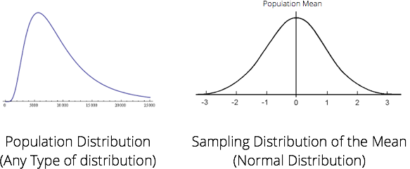
- The mean of the sampling distribution will cluster around the population mean.
- The standard deviation of the population distribution is tied with the standard deviation of the sampling distribution. With the standard deviation of the sampling distribution and the sample size, we are able to calculate the standard deviation of the population distribution. The standard deviation of the sampling distribution is called the standard error.
Ok, so technically, how do calculating confidence intervals work?
Beer, beer, beer…
Let’s go back to the beer example from my previous post. Say we are studying the American beer drinkers and we want to know the average age of the US beer drinker population. We hire a firm to conduct a survey on 100 random American beer drinkers. From that sample, we get the following (totally made up) results:
- n (sample size):
100 - Standard Deviation of Age:
15 - Arithmetic Mean of Age:
40
What can we infer from the population with this information? Quite a lot, actually.
With this data at hand and based on what we learned about the CLT, our best guess is that the population mean is more or less equal to 40, the mean of our sample. However, how can we be confident about this number? What are the chances that we are wrong?
What is the probability that the mean age of the US beer drinker population is between 38 and 42? (I selected those values to keep the example simple. By the of the post, you should be able to calculate this for any range.)
Standard Error & Standard Deviation
Here’s an important bit information I haven’t provided you with yet. This formula describes the relation ship between the Standard Error of the Mean and the Standard Deviation of the Population. It is necessary to use this formula in order to calculate confidence intervals and margins of error.
Standard Error of the Mean = Standard Deviation of Population / √n
The challenge is that with the data provided above, neither do we have the Standard Error nor the Standard Deviation of the Population. To solve this, alternatively to the Standard Deviation of the Population, we can use our best estimator for that value. In this case, our best estimator is the sample standard deviation.
Standard Error of the Mean = 15 / √100 = 1.5
We now know that our best estimate for the Standard Error of the mean is 1.5. This is equivalent to saying the standard deviation of the sampling distribution of the mean is 1.5. This value is essential in calculating the probability of us being wrong.
Probability of an observation
Armed with the standard error, we can now calculate the probability of our population mean being between 38 and 42. When working with a distribution such as the normal distribution, we generally want to normalize absolute values in terms of standard deviations. What does the range of 2 year above and below our arithmetic mean represents in terms of standard deviation? We can normalize this range by diving the 2 years by the standard deviation. It represents 2 / 1.5 or 1.33 standard deviation above or below the sample mean.
Since the normal distribution is a distribution of probabilities and it has been studied extensively, there is a table called the Z-Table that documents the probability that a statistic is observed. With the Z-Table, we can easily know the probability that an observation will occur above or below a certain standard deviation. We can lookup the information in the Z-Table to understand the probability of an observation being within 1.33 standard deviations from our mean.
In this case, the table tells us that the probability that the mean age of the US beer drinker population is between 38 and 42 is 81.64%. This is similar to saying that we are confident at approximately 81.64% that the population is more or less 2 years of our sample mean. There you have it, a confidence interval and a margin of error.
This example if fairly simple, I agree. It’s important to remember that a good portion of the data scientist work is just arithmetic. Understanding the fundamentals is essential if you want to interpret data. It will also help you do a better job at teaching your colleagues about it. As a data scientist, a major part of your job is to communicate clearly statistical concepts to people with various level of statistical knowledge.